Chapter 3

Design High-Performing Architectures

AWS Certified Solutions Architect – Associate (SAA-C03) Study GuideBased on the official AWS SAA-C03 exam objectives

The Solutions Architect Associate exam doesn't just ask whether you can build something on AWS — it asks whether you can build something that performs. Domain 3, "Design High-Performing Architectures," carries 24% of your exam score, the second-largest domain on the test. Every question in this domain shares the same underlying logic: given a workload with specific performance requirements, pick the service, configuration, or scaling strategy that meets them at the lowest cost and least complexity.

What makes a system "high-performing" on AWS is rarely raw speed alone. It's throughput (how much work gets done per second), latency (how fast each unit of work completes), and the ability to hold both steady when demand spikes. Throughout this chapter you'll notice the same three design patterns repeating: scale horizontally by adding resources, cache aggressively so you do less work, and move compute and data closer to the people and processes that need them. These patterns show up in compute, storage, databases, caching, networking, and analytics — and the exam loves to test whether you recognize them in new situations.

This chapter walks through each major AWS service through a performance lens: how EC2 instances differ in their compute and networking capabilities, how storage services trade latency for throughput, how caching layers eliminate redundant work, how databases scale reads and writes, and how serverless and streaming services handle bursty demand. We'll include worked calculation examples and exam tips drawn from the kinds of scenario questions the real test asks.

Choosing the Right EC2 Instance

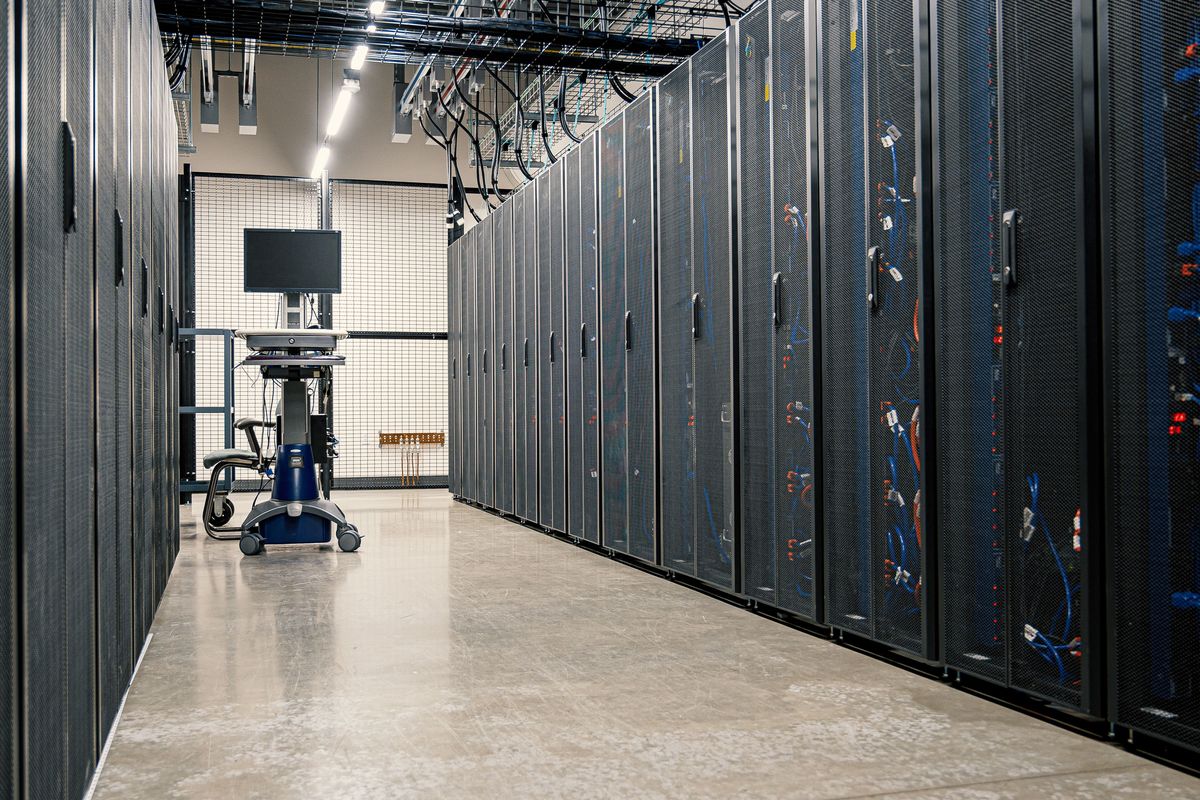
EC2 instances are virtual machines, but not all virtual machines are created equal. AWS organizes instances into families, and each family optimizes for a different bottleneck: raw compute, memory, storage I/O, networking, or graphics. The exam's favorite trick is describing a workload's symptoms and asking you to pick the family that fixes them.

The general-purpose families (T, M, and A-series) are the balanced all-rounders. T-series instances are burstable: they earn CPU credits while idle and spend them during bursts, which makes them perfect for development servers, small web apps, and anything with spiky-but-averaging-low usage. M-series instances give you a steady, consistent CPU for applications that can't tolerate throttling. If a question describes a workload that "runs at low utilization most of the time but occasionally spikes," the answer is almost always a T-family instance.

Compute-optimized instances (C-series) maximize CPU per dollar. Batch processing, media transcoding, high-performance web servers, machine learning inference, and dedicated gaming servers all live here. When a workload is "CPU-bound" — meaning the processor is the bottleneck — C-family is the move.

Memory-optimized instances (R-series, X-series) pack enormous RAM. In-memory databases, distributed caches, real-time analytics engines, and SAP workloads need memory far more than CPU. If the scenario says "the application loads a 200 GB dataset into memory," reach for R or X.

Storage-optimized instances (I, D, H-series) attach fast local NVMe SSDs — these are the "instance store" volumes we'll discuss in the storage section. They're built for workloads that hammer local disk: NoSQL databases like Cassandra, data warehousing, distributed file systems, and log processing. D-series specifically targets high disk throughput for dense storage workloads like Hadoop HDFS.

Accelerated-computing instances (P, G, Inf, Trn-series) attach GPUs or custom AI chips. Machine learning training, graphics rendering, and video encoding belong here.

Network Performance: ENA and EFA

Two networking technologies appear regularly on the exam: ENA (Elastic Network Adapter) and EFA (Elastic Fabric Adapter). Don't confuse them — they solve very different problems.

ENA is the standard high-performance network interface on modern EC2 instances, delivering up to 100 Gbps of bandwidth with low latency and low jitter. It's enabled by default on most current-generation instances. For virtually every exam scenario involving ordinary networking throughput — faster web serving, bigger file transfers — ENA-backed instances are the answer.

EFA is a specialized network device for tightly coupled HPC and machine-learning workloads. Standard TCP/IP networking involves the operating system in every packet (the kernel copies data, handles interrupts), which adds latency. EFA bypasses the OS kernel entirely — a technique called OS bypass — letting applications talk directly to the network hardware. This matters when thousands of nodes must coordinate with microsecond-level latency, like MPI-based scientific simulations or distributed machine-learning training. EFA does not replace your network interface; it's an additional device you attach alongside a normal interface, and it only works with specific instance types.

Placement Groups: Controlling Instance Proximity

When you launch EC2 instances, AWS scatters them across its data-center hardware by default. That scattering protects you from a single hardware failure, but it also means instances might sit in different racks with several network hops between them. Placement groups let you control this tradeoff, and there are three strategies:

A cluster placement group packs instances into a single Availability Zone, physically close together — same rack or adjacent racks. Network latency between instances drops to single-digit microseconds and throughput can hit 10 Gbps (more on ENA-backed types). The exam loves this for "HPC application that needs low-latency, high-throughput communication between nodes." The tradeoff: putting all instances in one AZ and one physical neighborhood reduces fault tolerance — a single rack failure can take out the whole cluster.

A spread placement group does the opposite: it places at most one instance per underlying physical host, spreading them across distinct racks. If the scenario involves "a small number of critical instances that must be isolated from each other to survive hardware failure" — think a handful of database primary nodes — spread is the answer. It's limited to a maximum of seven instances per AZ.

A partition placement group is the middle ground, designed for large distributed systems like Hadoop, Cassandra, and Kafka. Instances are divided into partitions (up to 7 per AZ), and each partition runs on separate racks. Data replication across partitions survives rack failures, while keeping instances in the same partition close together. When a question describes a "large distributed workload" (dozens or hundreds of nodes) that needs "isolation from correlated hardware failures," partition is the right choice.

Storage Performance: EBS, Instance Store, EFS, and FSx

Block storage on EC2 comes from two places: EBS volumes (network-attached, persistent) and instance store volumes (physically attached to the host, ephemeral). The exam tests whether you know which to use and how to tune each.

EBS Volume Types

EBS offers four volume types, split into SSD-backed (performance) and HDD-backed (throughput) categories:

gp3 (General Purpose SSD) is the default workhorse: a baseline of 3,000 IOPS and 125 MB/s throughput per volume, with both IOPS and throughput independently adjustable (up to 16,000 IOPS and 1,000 MB/s). It handles boot volumes, development environments, and low-latency interactive apps. You pay only for what you provision, so gp3 replaced gp2 as the sensible default.

io2 (Provisioned IOPS SSD) is for I/O-intensive workloads that need sustained, predictable performance: large databases like Oracle, SAP HANA, or high-transaction SQL Server. It delivers up to 64,000 IOPS per volume with a 99.999% durability SLA (versus 99.8–99.9% for gp3). io2 Block Express pushes that to 256,000 IOPS on the largest Nitro instances.

st1 (Throughput Optimized HDD) is for big-data workloads that stream large sequential reads and writes: log processing, data warehouses, ETL pipelines. It provides up to 500 MB/s per volume at the lowest cost per gigabyte.

sc1 (Cold HDD) is the cheapest option, for infrequently accessed data where throughput matters more than latency — file servers, archival staging.

A critical exam concept is provisioned IOPS: with gp3 and io2, you can specify exactly how many IOPS you need, independent of volume size. When a question says "the database needs 20,000 IOPS but only 500 GB of storage," that's a provisioned-IOPS scenario — io2 (or gp3 with provisioned IOPS, which is cheaper but caps at 16,000). Older gp2 tied IOPS to volume size (3 IOPS per GB), and the exam still asks about this behavior: on gp2, to get more IOPS you must create a bigger volume, which is exactly the wasteful pattern gp3's independent provisioning fixes.

You can also boost EBS performance by striping multiple volumes in RAID 0 for combined throughput, using EBS-optimized instances (which reserve dedicated network bandwidth for EBS traffic so storage I/O doesn't fight application traffic), and pre-warming volumes restored from snapshots.

Instance Store: Ephemeral Local Speed

Instance store volumes are physically attached to the host machine — NVMe SSDs on storage-optimized instances. They're extremely fast (hundreds of thousands of IOPS, microsecond latency) and free, but ephemeral: the data is lost if the instance stops, terminates, or the host fails. Use instance store for temporary data — caches, buffers, scratch space, replication data that exists elsewhere. Never put the only copy of anything important on instance store.

EFS Throughput Modes

Amazon EFS is a managed NFS file system shared across many EC2 instances — the exam's go-to answer for "shared file storage for Linux workloads" (content repositories, web-server farms, dev environments). EFS performance has two dimensions: throughput mode and performance mode.

Bursting throughput gives each file system a baseline throughput proportional to its size, plus burst credits for spikes — fine for typical workloads. Provisioned throughput lets you specify a fixed throughput level (up to 10+ GB/s with read access) regardless of file-system size, which is what you choose when a workload "needs 500 MB/s of throughput but only stores 100 GB" — the classic provisioned-throughput exam scenario. Elastic throughput automatically scales throughput up and down with actual usage, with no provisioning and no management; it's the simplest choice for spiky, unpredictable workloads.

Performance mode is separate: General Purpose (default, lowest latency, great for most files) versus Max I/O (higher throughput and IOPS for massively parallel workloads, with slightly higher latency). Note that once you pick Max I/O you can't change it back — the exam occasionally tests this.

FSx Variants

Amazon FSx provides fully managed third-party file systems. The exam expects you to match each variant to its use case:

• FSx for Windows File Server: native Windows SMB file shares with Active Directory integration. The answer for "Windows file shares that need AD authentication."
• FSx for Lustre: a parallel file system built for HPC — sub-millisecond latencies, massive throughput. The answer for "HPC scratch storage" or "machine-learning training data." It integrates natively with S3, so you can process S3 datasets at Lustre speeds and write results back.
• FSx for NetApp ONTAP: enterprise NetApp features (snapshots, cloning, replication) for workloads migrating from on-premises NetApp arrays.
• FSx for OpenZFS: managed ZFS for Linux workloads needing data compression, snapshots, and high performance.

Object Storage Performance: S3

S3 is already massively scalable — it can handle thousands of requests per second per prefix automatically. But several features exist to push S3 performance further, and the exam tests each one.

Multipart Upload

A single PUT request to S3 tops out at 5 GB, but more importantly, uploading one large file in a single stream is slow and fragile: one network hiccup restarts the whole thing. Multipart upload splits an object into parts (each 5 MB to 5 GB, up to 10,000 parts), uploads them in parallel, and S3 assembles them. It's required for objects over 5 GB and recommended for anything over 100 MB. The exam asks about this directly: "uploading 50 GB video files is slow and unreliable" → use multipart upload. It also parallelizes downloads via byte-range fetches.

Transfer Acceleration

S3 Transfer Acceleration routes uploads through the CloudFront edge network: instead of sending data across the public internet to the bucket's region, clients upload to the nearest edge location, and AWS's private backbone carries it the rest of the way. This helps most for clients far from the bucket region on congested public internet. The tradeoff: it costs extra, so the exam expects you to weigh it against alternatives like multipart upload. A question about "users in Australia uploading to a bucket in us-east-1" is a classic Transfer Acceleration scenario.

S3 Select and Performance Patterns

S3 Select lets you retrieve only a subset of an object's data using SQL expressions — instead of downloading a 10 GB CSV to find matching rows, S3 filters server-side and returns kilobytes. For analytics queries against large flat files, this cuts both transfer time and cost dramatically. Its sibling, S3 Glacier Select, does the same against archive storage.

Two more S3 performance patterns the exam loves: S3 batch operations for performing the same operation (copy, tag, restore) across millions of objects, and the general guidance that S3 now automatically scales to very high request rates — you no longer need to randomize key prefixes the way old documentation suggested.

Content Delivery and Global Acceleration

CloudFront Caching

CloudFront is AWS's content delivery network: a global fleet of edge locations that cache your content close to users. When a user requests content, CloudFront serves it from the nearest edge cache; only cache misses travel back to the origin (your S3 bucket, ALB, or EC2 instance). This cuts latency dramatically for global audiences and reduces load on your origin.

The performance lever you control is the TTL (time-to-live): how long CloudFront keeps an object cached before re-checking the origin. Longer TTLs mean more cache hits and less origin load, but staler content. For static assets (images, CSS, JavaScript), set long TTLs and use versioned filenames (app-v2.js) so updates bypass the cache problem entirely. For dynamic or personalized content, use short TTLs or bypass caching. Cache invalidations force fresh fetches but cost money and take minutes — the exam wants you to prefer versioning over invalidation.

Origin failover and Lambda@Edge/CloudFront Functions extend the story: the former routes to a backup origin if the primary is unhealthy, while the latter run code at the edge for request/response manipulation (URL rewrites, header injection, A/B testing) with minimal latency. CloudFront Functions are lighter and cheaper for simple manipulations; Lambda@Edge supports full Node.js/Python runtimes for heavier logic.

Global Accelerator

AWS Global Accelerator is often confused with CloudFront, but it accelerates anything, not just cacheable HTTP content. It gives your application two static anycast IP addresses; user traffic enters the AWS global network at the nearest edge location and rides the private backbone to your endpoint — ideal for TCP/UDP workloads like gaming, VoIP, or APIs where every millisecond counts and content can't be cached. It also provides instant regional failover: health checks shift traffic to a healthy region in under a minute, without DNS propagation delays.

Caching: ElastiCache and DAX

Caching is the single highest-leverage performance technique in the Solutions Architect toolkit: store the result of expensive work in fast memory, and serve repeat requests from memory instead of redoing the work. A cache hit can turn a 200-millisecond database query into a 1-millisecond memory lookup, while simultaneously reducing load on the database so it scales further.

ElastiCache: Redis vs Memcached

Amazon ElastiCache offers two engines. They look similar — both are in-memory key-value stores — but the exam tests their differences relentlessly.

Redis is the feature-rich option: it supports complex data structures (lists, sets, sorted sets, hashes, streams), persistence (snapshots to disk), replication with automatic failover (Multi-AZ), pub/sub messaging, and transactions. Choose Redis when you need high availability, durability of cached data, leaderboards, session stores that must survive failover, or real-time messaging. Redis Cluster mode shards data across nodes for horizontal scaling of both memory and throughput.

Memcached is the simpler, leaner option: a pure in-memory cache with no persistence, no replication, and no complex data types — just key-value pairs. It shines when you need to scale a cache tier horizontally with minimal fuss, and each node is independent. Because Memcached clients do the sharding themselves, adding nodes linearly increases cache capacity. Choose Memcached for simple caching of database query results or HTML fragments where losing the cache on a node failure is acceptable (it just refills from the database).

The classic exam pattern is the lazy-loading (cache-aside) strategy: the application checks the cache first; on a miss, it reads from the database, writes the result to the cache with a TTL, and returns it. This keeps the cache populated only with data that's actually requested. Write-through caching (write to cache and database simultaneously) guarantees the cache is always fresh but adds latency to every write — appropriate when stale reads are unacceptable.

DAX: Caching for DynamoDB

DynamoDB Accelerator (DAX) is a fully managed, in-memory cache built specifically for DynamoDB — and it's the only cache that requires zero application changes to the DynamoDB API. You point your existing DynamoDB client at the DAX cluster endpoint, and it behaves exactly like DynamoDB, except reads that hit the cache return in microseconds instead of milliseconds.

Use DAX when a DynamoDB table is read-heavy with repeated reads of the same items — "millions of reads per second, mostly the same popular items" is the textbook scenario. It supports both write-through and write-around caching. Note that DAX only accelerates eventually-consistent reads; strongly consistent reads and writes still go to the table. If the exam describes a workload that needs microsecond read latency on DynamoDB with no code changes, DAX is the answer — not ElastiCache, which would require rewriting the data-access layer.

NoSQL at Scale: DynamoDB

DynamoDB is AWS's managed NoSQL database: single-digit-millisecond latency at any scale, with no servers to manage. Performance tuning in DynamoDB revolves around capacity modes, scaling, and data modeling.

Capacity Modes: On-Demand vs Provisioned

On-demand mode charges per request and scales instantly to any traffic level — perfect for new applications, unpredictable workloads, or spiky traffic where you can't forecast demand. You pay a premium per request for that flexibility.

Provisioned mode lets you specify read and write capacity units (RCUs/WCUs) per second, and it's cheaper when traffic is predictable. Auto scaling adjusts provisioned capacity up and down based on actual utilization, so you get cost efficiency without manual tuning — the exam's favorite answer for "predictable baseline with occasional spikes, minimize cost." One RCU handles one strongly consistent read (or two eventually consistent reads) per second for items up to 4 KB; one WCU handles one write per second for items up to 1 KB. Larger items consume proportionally more units.

Partition Keys, GSIs, and LSIs

DynamoDB distributes data across partitions based on the partition key. Performance collapses when one partition key value gets disproportionate traffic — the infamous hot partition problem. The exam tests this with scenarios like "all writes use the same partition key (e.g., today's date)" — the fix is to design a partition key with high cardinality (user ID, device ID) or add a random suffix (write sharding) to spread the load.

Global Secondary Indexes (GSIs) let you query on attributes other than the table's keys. Each GSI has its own partition key, its own provisioned throughput, and is updated asynchronously (eventual consistency). GSIs are the answer to "we need to query the table by a different attribute." Local Secondary Indexes (LSIs) share the table's partition key but offer an alternative sort key; they must be created at table-creation time and share the table's throughput. The exam distinction: GSI = different partition key, created anytime, own throughput; LSI = same partition key, created only at table creation, shares throughput.

Additional DynamoDB performance features worth knowing: DynamoDB Streams capture item-level changes for triggering Lambda functions (event-driven architectures); global tables replicate data across regions for multi-region active-active workloads with low-latency local reads; and Time to Live (TTL) automatically deletes expired items, which keeps tables lean and queries fast.

Relational Databases: RDS, Aurora, and Redshift

RDS Read Replicas and RDS Proxy

Amazon RDS runs managed relational databases (MySQL, PostgreSQL, MariaDB, Oracle, SQL Server). When read traffic overwhelms the primary instance, read replicas offload it: asynchronous copies of the primary that serve read queries. You can create up to 15 read replicas per primary (5 for Oracle/SQL Server), place them in other AZs or regions, and even promote one to standalone if the primary fails. The exam's classic scenario: "the application's read traffic has grown 10x, writes are unchanged" → add read replicas and split reads from writes at the application level. Remember the tradeoff: replication is asynchronous, so replicas lag slightly behind — fine for reporting and dashboards, wrong for "read-your-own-write" consistency needs.

RDS Proxy solves a different problem: connection storms. Serverless applications and auto-scaled fleets can open thousands of database connections, exhausting the database's connection limit and wasting memory on idle connections. RDS Proxy sits between the application and the database, maintaining a pool of long-lived connections and multiplexing application connections onto them. It also makes failovers faster (typically under 30 seconds versus minutes) because the proxy holds the endpoint steady while swapping the underlying connection. "Lambda functions opening too many connections to RDS" → RDS Proxy, almost every time.

Aurora Endpoints

Amazon Aurora (MySQL- and PostgreSQL-compatible) is AWS's cloud-native relational database, and its endpoint architecture is heavily tested:

• The cluster endpoint always points to the current primary (writer) instance — use it for all writes.
• The reader endpoint load-balances connections across all read replicas — use it for read scaling.
• Custom endpoints let you define your own subset of instances — for example, routing expensive analytics queries to a dedicated large replica so they don't slow down the replicas serving the application.

Aurora storage auto-scales from 10 GB to 128 TB, replicates six ways across three AZs, and supports up to 15 low-latency read replicas. Aurora Serverless pauses during idle periods and scales capacity automatically — ideal for intermittent or unpredictable workloads. Aurora Global Database replicates to other regions with typically under a second of lag for disaster recovery and low-latency global reads.

Redshift Distribution Styles

Amazon Redshift is a petabyte-scale data warehouse, and its performance hinges on distribution styles — how table rows are spread across compute nodes:

• KEY distribution places rows with the same distribution-key value on the same node. Use it for large tables that are frequently joined on that key: co-located joins avoid expensive cross-node data shuffling. Both sides of a frequent join should use the same distribution key.
• ALL distribution copies the entire table to every node. Use it for small dimension tables (a few million rows) that join against everything — every node can join locally with zero network traffic.
• EVEN distribution spreads rows round-robin across nodes. Use it when a table isn't joined often or has no good key; it balances load but forces network shuffling on joins.
• AUTO distribution (the default) lets Redshift choose and adjust the style based on observed query patterns — the right answer when the exam doesn't give you enough detail to pick manually.

Sort keys are the companion concept: they order rows on disk so range queries (WHERE date BETWEEN ...) skip entire blocks. Compound sort keys serve multi-column filters; interleaved sort keys help when filters vary.

Serverless Performance: Lambda and API Gateway

Lambda: Memory, CPU, and Cold Starts

Lambda performance has one golden rule the exam tests constantly: CPU scales with memory. When you allocate more memory to a function (128 MB to 10 GB), you get proportionally more CPU power and network bandwidth. A compute-heavy function given 3 GB of memory runs dramatically faster than the same function at 128 MB — and because Lambda bills by gigabyte-seconds, the faster execution often reduces total cost. The exam scenario "the Lambda function is slow and timing out on heavy computation" is usually solved by increasing memory, not by rewriting code.

Cold starts are the other major concept: when Lambda needs a new execution environment (first invocation, or scaling up), it must initialize the runtime — adding hundreds of milliseconds to seconds of latency. Provisioned concurrency keeps a set number of environments warm and ready, eliminating cold starts for latency-sensitive applications. It costs money even when idle, so use it only where consistent low latency matters (user-facing APIs, real-time processing). SnapStart (for Java functions) takes a snapshot of an initialized execution environment and restores it in milliseconds — a cheaper cold-start fix, but only for Java runtimes.

Lambda scaling itself is automatic and aggressive — up to 1,000 concurrent executions by default (soft limit, increasable). Each concurrent execution is isolated. For functions that must not scale (to protect a downstream database), reserved concurrency caps the maximum; for functions sharing an account's pool, unreserved concurrency is the remainder.

API Gateway Caching

API Gateway fronts your APIs (Lambda, HTTP backends, AWS services). Its performance lever is caching: API Gateway can cache endpoint responses in memory, serving repeat requests without invoking the backend at all. You enable caching per stage, choose a cache capacity, and set a TTL. Cache keys can include query strings, headers, and path parameters so different requests don't collide.

The exam scenarios are straightforward: "the API is throttled / Lambda costs are spiking from repeated identical requests" → enable API Gateway caching. It's also the answer for "reduce latency for frequently requested, slowly changing data" (product catalogs, reference data). Note the cost: caching adds a per-hour charge based on cache size, so it's worth it only when the backend savings exceed it.

Additional API Gateway performance notes: use regional endpoints for clients in the same region and edge-optimized endpoints (CloudFront-backed) for geographically distributed clients; throttling and usage plans protect backends from traffic spikes; and request/response transformation and payload compression reduce transfer sizes.

Streaming and Messaging: Kinesis, MSK, and SQS

Kinesis Data Streams vs Firehose vs MSK

The exam treats the Kinesis family as a matching exercise, and getting the match right is worth several questions:

Kinesis Data Streams (KDS) is real-time streaming with full control: you provision shards (each handles 1 MB/s in and 2 MB/s out), consumers read with sub-second latency, and data is retained up to 365 days for replay. Use KDS when you need real-time processing with custom consumers — fraud detection, live dashboards, clickstream analysis. Enhanced fan-out gives each consumer dedicated 2 MB/s throughput so multiple consumers don't compete. Scaling means adding shards (or using on-demand mode for automatic scaling).

Kinesis Data Firehose is the zero-management delivery service: it captures streaming data and automatically delivers it to destinations — S3, Redshift, OpenSearch, Splunk, or HTTP endpoints. No shards to manage, no consumers to write; it buffers, batches, compresses, and can transform data with Lambda en route. Use Firehose when the goal is "get streaming data into storage/analytics with no code" — the classic "ingest clickstream data into S3 for Athena queries" scenario. Near-real-time (buffered by time or size, typically 60 seconds+) rather than true real-time.

Amazon MSK (Managed Streaming for Apache Kafka) is managed Apache Kafka for teams that need Kafka's ecosystem — exactly-once semantics, stream processing with Kafka Streams, or existing Kafka tooling and expertise. It's heavier to operate than Kinesis but offers full Kafka compatibility.

SQS deserves a mention here as the exam's decoupling workhorse: a fully managed message queue that absorbs traffic spikes between producers and consumers. Standard queues offer nearly unlimited throughput with at-least-once delivery; FIFO queues guarantee ordering and exactly-once processing at lower throughput (300 messages/s, or 3,000 with batching). "Smooth out spiky traffic to a backend that can't scale fast enough" → SQS buffer in front of it.

Analytics Performance: EMR, Athena, and Glue

EMR, Athena, and Glue Basics

For big-data analytics, the exam wants you to match the tool to the performance profile:

Amazon EMR runs managed Hadoop, Spark, Hive, and Presto clusters. Its performance advantage is elasticity: spin up hundreds of nodes for a nightly job, then terminate them. Use Spot Instances for task nodes to cut costs up to 90%, keep the cluster in the same AZ as your S3 data, and use the latest generation instances. EMR is the answer for "large-scale distributed processing with full framework control" — ETL pipelines, machine-learning feature engineering, log analysis at terabyte scale. EMR Serverless removes even cluster management for Spark and Hive jobs.

Amazon Athena is serverless SQL on S3: point it at your data lake and run queries with no infrastructure. Performance comes from data layout, not tuning: partition your data (by date, region), use columnar formats like Parquet or ORC instead of CSV/JSON, and compress files. These three practices can cut query time and cost by 10–100x because Athena charges per byte scanned. S3 Select (from earlier in this chapter) is Athena's lightweight cousin for simple filtering.

AWS Glue is the serverless ETL service: it discovers your data with crawlers, catalogs it in the Data Catalog, and runs Spark-based transform jobs. Its performance features include job bookmarks (process only new data instead of reprocessing everything), auto scaling of workers, and Glue DataBrew for visual data preparation. The exam scenario "nightly ETL from S3 to Redshift with minimal management" points to Glue.

Tying It Together: The Performance Design Patterns

Step back and notice what this chapter keeps repeating. Every high-performing architecture on AWS combines a few moves: choose the resource matched to the bottleneck (instance family, volume type, distribution style); scale horizontally instead of vertically (read replicas, shards, auto scaling); cache at every layer (CloudFront, ElastiCache, DAX, API Gateway); move data closer to consumers (edge locations, Global Accelerator, Transfer Acceleration, global tables); and batch or filter work before doing it (multipart upload, S3 Select, Glue bookmarks, Athena partitioning). The exam's scenario questions are variations on these themes — identify the bottleneck, then apply the matching pattern. Master that reflex and Domain 3 becomes the most predictable 24% of your score.

End-of-Chapter Test

1. A company runs a tightly coupled HPC simulation using MPI across 200 EC2 instances. The simulation requires microsecond-level network latency between nodes with minimal operating system overhead. Which networking solution should the architect choose? A) Enable ENA on all instances for up to 100 Gbps bandwidth B) Attach an Elastic Fabric Adapter (EFA) to the instances C) Place the instances in a spread placement group D) Use Global Accelerator to route traffic between instances

2. A database workload requires 20,000 provisioned IOPS but only 600 GB of storage. The workload needs sustained, predictable I/O performance with the highest durability SLA. Which EBS volume type is most appropriate? A) gp3 with 20,000 provisioned IOPS B) io2 with 20,000 provisioned IOPS C) st1 with 600 GB provisioned D) gp2 with a 6,667 GB volume

3. A web application stores user-uploaded videos averaging 8 GB each in S3. Users report that uploads frequently fail on slow connections and must restart from the beginning. What should the architect implement to fix this? A) Enable S3 Transfer Acceleration on the bucket B) Use S3 multipart upload for the video files C) Enable S3 Versioning on the bucket D) Move the videos to EFS

4. An application performs millions of DynamoDB reads per second, mostly against the same popular items, and needs microsecond read latency without changing any application code. Which solution meets these requirements? A) Add an ElastiCache for Redis cluster in front of DynamoDB B) Switch the table to provisioned capacity mode with auto scaling C) Add a DynamoDB Accelerator (DAX) cluster in front of the table D) Create a global secondary index on the popular attributes

5. A Lambda function processes images and consistently runs for 9 seconds at 256 MB of memory, occasionally timing out at the 10-second limit. The workload is CPU-bound. What is the most effective first step? A) Enable provisioned concurrency for the function B) Increase the function's memory allocation C) Enable SnapStart for the function D) Split the function into smaller Step Functions tasks

6. A company needs Windows file shares with Active Directory integration for its on-premises users, migrated to AWS with minimal changes. Which FSx variant should the architect choose? A) FSx for Lustre B) FSx for Windows File Server C) FSx for NetApp ONTAP D) FSx for OpenZFS

7. An e-commerce API backed by Lambda receives thousands of identical product-catalog requests per minute. Backend costs are rising and p99 latency is degrading. What is the simplest effective fix? A) Enable API Gateway caching for the catalog endpoints B) Add RDS Proxy between Lambda and the database C) Increase Lambda memory to 10 GB D) Deploy the API in a cluster placement group

8. A Redshift data warehouse has a 500 GB fact table frequently joined to a 2 GB dimension table on customer_id. How should the architect configure distribution styles for best join performance? A) KEY distribution on customer_id for the fact table, ALL distribution for the dimension table B) EVEN distribution for both tables C) ALL distribution for the fact table, KEY distribution for the dimension table D) AUTO distribution for both tables with no sort keys

9. A company needs to ingest a continuous stream of clickstream events and deliver them to S3 for Athena queries, with minimal operational management and no custom consumer code. Which service should the architect choose? A) Kinesis Data Streams with enhanced fan-out B) Kinesis Data Firehose C) Amazon MSK D) SQS FIFO queues

10. A mobile gaming company serves players worldwide with a real-time multiplayer backend using custom TCP protocols. Content cannot be cached, and the game needs fast regional failover without DNS delays. Which solution should the architect choose? A) CloudFront with Lambda@Edge B) AWS Global Accelerator C) S3 Transfer Acceleration D) Route 53 latency-based routing alone

11. A Lambda-based order processing system opens thousands of simultaneous connections to an RDS MySQL database during sales events, exhausting the database connection limit. What should the architect implement? A) Add RDS read replicas B) Deploy RDS Proxy in front of the database C) Move the database to DynamoDB on-demand mode D) Increase the RDS instance size

12. An Athena query scanning 500 GB of CSV logs in S3 is slow and expensive. The logs are queried mostly by date range. Which combination of changes will most improve performance and cost? A) Convert the data to Parquet format, compress it, and partition by date B) Move the data to EBS io2 volumes and query from EC2 C) Enable S3 Transfer Acceleration on the bucket D) Create a global secondary index on the date attribute

Answer Key

1. B — EFA provides OS-bypass networking for tightly coupled HPC/ML workloads needing microsecond latency; ENA is general-purpose bandwidth, and spread placement groups hurt rather than help latency. 2. B — io2 supports 20,000 provisioned IOPS (gp3 caps at 16,000) with a 99.999% durability SLA for sustained I/O-intensive database workloads. 3. B — Multipart upload splits large objects into parallel parts that can be retried individually, fixing slow, fragile large-file uploads. 4. C — DAX is a drop-in in-memory cache for DynamoDB delivering microsecond reads with no application code changes; ElastiCache would require rewriting the data-access layer. 5. B — CPU scales with memory in Lambda, so increasing memory speeds up CPU-bound functions and often reduces cost via shorter billed duration. 6. B — FSx for Windows File Server provides native SMB shares with Active Directory integration for Windows workloads. 7. A — API Gateway caching serves repeat identical requests from memory without invoking Lambda, cutting both cost and latency for slowly changing data. 8. A — KEY distribution co-locates the fact table's join rows on the same nodes, while ALL distribution replicates the small dimension table everywhere so joins happen locally with no network shuffling. 9. B — Firehose delivers streaming data to S3 with zero consumer code or shard management; Data Streams and MSK require custom consumers. 10. B — Global Accelerator routes non-cacheable TCP/UDP traffic over AWS's private backbone with static IPs and sub-minute regional failover. 11. B — RDS Proxy pools database connections and multiplexes thousands of application connections onto a few long-lived ones, solving connection exhaustion. 12. A — Parquet (columnar) plus compression plus date partitioning lets Athena scan far fewer bytes, which directly cuts both query time and per-byte-scanned cost.